
The unknown “Format as conditions” in Excel can really impress.
Microsoft Excel's Conditional Formatting feature is extremely useful, it can boost your spreadsheet productivity, impress your bosses (or professors) and make things a little more fun at the same time.
A few words about Microsoft Excel
Much of Excel's power lies behind its formulas and rules that help you manipulate data and information automatically, regardless of the data you enter into the spreadsheet.
Microsoft Excel formulas can do almost anything. In this article, you will learn how powerful a tool it can be formatting conditional, and what you can do with it..
Conditional formatting with Excel formulas
One of the tools that people don't use often enough is the Conditional formatting. By using Excel formulas, rules, or a few very simple settings, you can turn a spreadsheet into an automated dashboard.
To go to Conditional Formatting, just click on the “Main” tab and click on its icon lineof the “Conditional Formatting” tools located in the “Styles” group.
In the Conditional Formatting section, there are several options. Most of these are outside the scope of this particular article, but in general almost all of them are related to episignalness, coloring or shading cells based on the data in that cell.
The most common use of conditional formatting is perhaps to turn a cell red or green using the “less than” or “greater than” formulas. It is a quick form of the IF-THEN-ELSE command, as for example: IF 'a cell' is greater than 'a number' THEN make red ELSE make green.
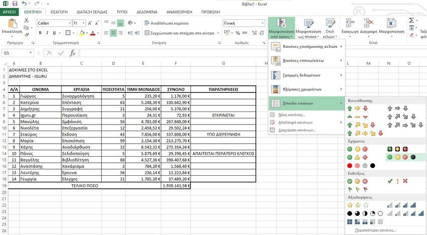
One of the least used conditional formatting tools is the choice “Image Sets”, which offers a great set of icons that you can use to add an icon to an Excel data cell based on some rule.
You should first choose some ready-made images and also choose a set of cells.
Then you will click on “Manage rules” (Manage Rules), you will be taken to “Show conditional formatting rules” (Conditional Formatting Rules Manager).
Depending on the data you select, you will see the cells indicated in the Manager window with the set of icons you just selected.
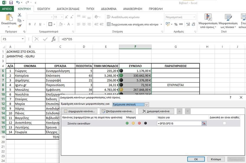
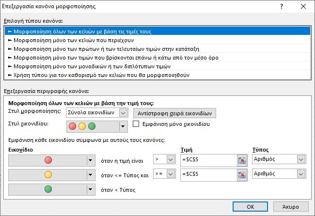
When you click Edit Rule, you'll see the dialog where the magic happens.
Here you can create the logic formula and equations that will display the dashboard icon you want.
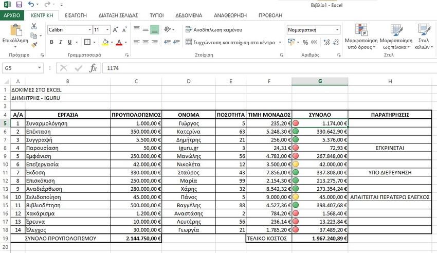
The example table below will show the costs for different tasks against the budget. If you go over budget, a red light will appear. If the cost is equal to the budget it will turn yellow. If you are below budget it will be green.
The formatting of each cell can be transferred to the other with the formatting brush and with minor modifications. If you do this in an entire column, each cell in that column will change color like a traffic light, depending on the cost of each task.
This way you and your intemperates can have immediate supervision if a price "hits" and you need to focus on it.
As a visual medium it is very pleasant and has many ready-made images to add to your cells.